| Information |  | |
Derechos | Equipo Nizkor
| ||
| Information | | |
Derechos | Equipo Nizkor
| ||
Apr14
IMF Working Paper
Transmission of Financial Stress in Europe:
The Pivotal Role of Italy and Spain, but not Greece
Prepared by Brenda González-Hermosillo and Christian Johnson |1|
Contents II. Identifying Systematic and Idiosyncratic Risk
A. Data Description
B. Causality TestsIII. Competing Empirical Models
A. Deterministic Volatility Models
B. Stochastic Volatility Model
C. Stochastic Volatility AnalysisA. Stability Analysis
B. Extending the Model Through October 2012 and Explaining Spanish and Italian Sovereign Credit Default SwapTables
1. Stylized Facts for Sovereign Credit Default Swap, TED Spread, and VIX
2. Causality Tests for Sovereign Credit Default Swap, TED Spread, and VIX
3. Estimation Results for the German Sovereign Credit Default Swap Spreads: Volatility ModelsFigures
1. Sovereign Credit Default Swaps, TED Spread, and VIX Index
2. Determinants of German Sovereign Credit Default Swap Volatility: Stochastic Volatility Model
3. Sovereign Credit Default Swaps
4. Volatility Decomposition Using Rolling Window Data
5. Volatility Decomposition: Germany, Italy, and Spain
Abstract This paper proposes a stochastic volatility model to measure sovereign financial distress. It examines how key European sovereign credit default swap (CDS) spreads affect each other; specifically, the paper analyses the volatility structure of Germany, Greece, Ireland, Italy, Spain and Portugal. The stability of Germany is a close proxy for the resilience of the euro area as markets use Germany's sovereign CDS as a hedge for systemic risk. Although most of the CDS changes for Germany during 2009-12 were due to idiosyncratic factors, market developments in Italy and Spain contributed significantly, likely due to their relative importance in the region. Changes in Greece's sovereign CDS had no significant effect on Germany's sovereign CDS despite initial widespread concerns about such linkages. Spain and Italy show a notable co-dependence in explaining each other's volatility while Germany also plays an important role. It is found that extreme bad news led to persistent and nearly permanent effects on the stochastic volatility of European sovereign CDS spreads.
I. Introduction On July 26, 2012, Mario Draghi, President of the European Central Bank (ECB), announced a commitment to do "whatever it takes" to counter perceptions of a euro area break-up by buying a potentially unlimited amount of government debt through the Outright Monetary Transactions (OMT) program. The motivation for this unconventional move was to reduce the interest rate premia demanded by financial markets for some peripheral countries in Europe, which were viewed by some as not justified by economic fundamentals and largely as a result of contagion.
Indeed, since the time when Greece revealed a much larger-than-expected fiscal deficit of 12.5 percent of GDP in October 2009, default concerns about Greece began to affect the sovereign credit default swap (SCDS) spreads and the cost of borrowing of other peripheral countries in Europe. Greece eventually had to be rescued, twice in 2010 and 2011. Ireland and Portugal also had to adopt a stabilization program endorsed by the troika, the European Commission (EC), the European Central Bank (ECB), and the International Monetary Fund in 2011. On and off since then, concerns about contagion have been generally viewed as driving, at least in part, SCDS spreads and the cost of financing for fiscally vulnerable European countries. Moreover, concerns about spillovers across countries and higher costs of funding for sovereigns and corporations partly underpin policies attempting to limit trading in European-referenced SCDS. This was the rationale for the European Union's ban on "naked" (i.e., without a corresponding offsetting position in the underlying debt) protection buying of SCDS that went into effect on November 1, 2012. |2|
Overall, a key lesson from recent financial crises is that contagion and spillovers are important factors that can rapidly transform idiosyncratic events into systemic crises. This is evident from a number of recent episodes of financial crises, including the recent global financial crisis that began in 2007-08. |3| Clearly, growing interconnectedness and risk of spillovers and contagion across the world have become a growing source of systemic risk. From a policy perspective, macro-prudential measures have been recently proposed to limit, inter alia, the effects of contagion and spillover risks during periods of stress.
Concerns about contagion have been abundant during the recent global financial crisis as it underwent several stages. First, the buildup of funding pressures beginning in early 2007 led to the systemic crisis that was exposed in the autumn of 2008 after the collapse of Lehman Brothers. This was followed by a systemic response phase that began in 2009 in a number of countries through either direct or indirect government guarantees of banks, or through outright purchases of financial assets that had become illiquid when their market values became uncertain. During this phase, concerns about contagion and spillovers provided a justification for policymakers to become the buyers/dealers or guarantors of last resort for the financial system. As the balance sheets of a number of these governments deteriorated, in part as a consequence of the transfer of risk from the financial sector to the sovereign, contagion and spillovers further became a major concern for some countries as it highlighted a further loop between sovereigns and the financial sector. Some of the fiscally weaker countries in Europe were affected the most. In each case, the requests for external financial assistance for Greece, Ireland and Portugal during 2010-11 were coupled with market concerns that other European countries could become affected by contagion.
While, indeed, all aspects of the recent global financial crisis have yet to be fully understood, the need to better comprehend contagion and spillovers is highlighted by recent events in Europe. Most notably, Greece has fared the worst since Standard's & Poor downgraded it in December 2009. In 2011, and after lengthy negotiations with creditors, Greece's external debt was written down significantly. Initially, commentators questioned how Greece's problems could affect creditor banks which were largely concentrated in the European core countries (mainly Germany and France). Later, in late-2011 when the European Central Bank's introduced its first Long-Term Refinancing Operation (LTRO), and subsequently in mid-2012 after the second ECB's LTRO injected close to 1 trillion euros in total, concerns about other large European countries such as Italy and Spain began to surface. Indeed, it was not until mid-2012 that European officials recognized the implications of contagion and openly discussed the possibility of a Greek exit from the euro for the first time. In the first half of 2012, Spain's market access and increased cost of funding renewed attention to the potential spillovers to Europe's core and, indeed, the stability of the euro area.
Contagion can materialize through several channels, some of which can be observed through asset prices or returns, or through their volatility. Of course, not all changes in asset prices or volatility are associated with contagion, as some portion of these movements may correspond to an idiosyncratic component. This paper takes a different approach from others that have empirically examined contagion. |4| In particular, it uses a stochastic volatility technique to decompose SCDS into systematic and idiosyncratic factors. To our knowledge, this paper is the first contribution to the literature on financial contagion that identifies a systematic-idiosyncratic decomposition modeling of risk using SCDS jointly with a stochastic volatility model.
While the existence of contagion is now hardly disputed, the actual mechanisms for contagion are less well understood and difficult to measure. These channels include:
- Contagion from one country to other sovereigns: Countries exhibiting similar weaknesses to the source country are affected through confidence effects. This increases their funding costs and worsens the sustainability of their debt dynamics, potentially accelerating downgrades in a self-fulfilling way. Discrimination across countries based on differences in fundamentals weakens once confidence erodes.
- Contagion to asset prices and risk appetite: Sovereign stress could propagate more broadly to asset markets, leading to a sudden rise in risk premia, a fall in asset prices, higher volatility and a drying up of liquidity. Measures of global market conditions can therefore play a role in the propagation mechanism. |5|
- Contagion to liquidity and funding markets: a risk of a generalized retreat from risk throughout markets can create an adverse cycle of worsening liquidity problems. Illiquid conditions can lead to solvency issues. For example, interbank lending markets could become dysfunctional and lead to credit lines being cut.
- Contagion between the financial sector and the sovereign: The banking sector can be heavily affected through funding pressures and capital charges emanating from losses on holdings of government bonds. The cost of financing of the sovereigns could also affect the corporate sector.
Evidently, these mechanisms can be very complex and it is often difficult to separate fundamental factors from induced propagation mechanisms. This paper examines a basic stylized or 'reduced form' model which abstracts from the specific intricate connections, focusing on separating the basic systematic factors from the idiosyncratic components during the European sovereign crisis. That is, looking at the drivers of volatility (lagged and contemporaneously through deterministic and stochastic specifications) that are driven by own factors specific to the sovereign risk of the country in question vs. the factors stemming from other countries.
This paper investigates empirically the effects of spillovers from the key euro area countries to Germany as the core country in the euro area and vice versa. Germany's CDS are of special interest because these instruments are often viewed by markets as instruments to hedge systemic risk in the euro area.
The data sample covers several periods. The first period covers February 2009 through April 2010, before concerns about some of the larger European countries were evident in press reports. We then extend the sample through July 2012 and then to October 2012 to check for stability and robustness. This allows us to present more robust results and question whether the recent concerns about some of the largest European countries were already priced-in by markets when all eyes appeared to be exclusively on Greece. The first period covers the time through which Greece requested financial assistance from the troika EC/EU/IMF. The extended sample period covers the time when Portugal and Ireland also requested financial support and there was rising speculation over Spain's need for potential assistance. During the latter period, Italy's high and volatile cost of funding was also a concern.
The analytical approach is based on daily data of SCDS as a measure of sovereign credit risk. The framework is a stochastic volatility model used to examine the dynamics of SCDS markets. The results suggest that, for the earlier period 2009-10 when observers were concerned almost exclusively about events in Greece, SCDS markets were already pricing-in potential problems in the largest European countries (namely, Italy and Spain) and the implications for the core. These effects are even stronger during the extended period through 2012.
A remarkable finding from this paper is the persistent and almost permanent effect that extreme bad news have on the stochastic volatility and, consequently, also on the change in SCDS spreads. Changes in the credit ratings of Greek sovereign debt, including news announced in the first quarter 2010 related to Greece's bailout package, had no statistical effect on Germany's SCDS. It is also interesting that the global (non-European) measures used as proxies for global market conditions (VIX and TED spreads) were not statistically significant in explaining Germany's SCDS dynamics. In fact, it would appear that Germany's SCDS dynamics are driven not only by idiosyncratic risk (reflecting its own macroeconomic and financial conditions), but also by market developments in Italy and Spain as measured by their SCDS spreads. The results suggest that these effects were evident as far back as 2009-10, even though they were not obvious from press reports at that time. These effects have become stronger since then.
One possible explanation for this is that Greece is seen as a country too small to affect Germany's risk profile. In contrast, Italy and Spain-being much larger economies-could potentially destabilize Germany or the euro area, even though their likelihood of running into financial difficulties was perceived by the markets as comparatively smaller, based on their SCDS spreads. The other potential (and complementary) explanation driving these results is the sheer size of CDS gross notional amounts outstanding, which place Italy and Spain as the two largest referenced entities with US$388 billion and US$212 billion, respectively, of outstanding SCDS contracts at end-2012. The growth of these two markets is also remarkable, as Spain was the fourth largest at end-2010. In contrast, Greece's CDS outstanding were US$77 billion at end-2010 or the 12th largest and it dropped out of the sample after March 2012 when Greece's debt sovereign restructuring was the largest in history. Germany's CDS gross notional amounts outstanding at end-2012 were the 5th largest in the market for all CDS (including sovereigns for other advanced and emerging market economies, and corporate firms). |6| The strong estimated impact of Italy and Spain on Germany may also capture the exposure of the latter to a break-up of the euro, reflecting euro-area systemic risks which would need to be tackled by systemic (i.e., euro-area wide) policy tools.
When the data sample is extended to October 2012, we find robust results that the volatility of Germany's SCDS is explained largely by idiosyncratic effects, but also by Italy and Spain's SCDS volatility (and not much else, including global market variables). However, the volatility of Spain and Italy's SCDS are affected by Germany's SCDS and each other's SCDS (and, again, not by much else). This is consistent with other observations of the so called "herding contagion" as a sharp simultaneous increase in sovereign yields across countries (Beirne and Fratzscher, 2012). Furthermore, our results suggest that there is high persistence in SCDS volatility during periods of stress. In other words, once things are seen as deteriorated, views do not appear to change easily. In terms of the economic interpretation, we see it as consistent with the view that Spain and Italy are key countries affecting the core of the euro area, which is Germany. At the same time, Germany is important for Spain and Italy because it is the benchmark (or risk-free country) in the euro area. But Spain and Italy are quite important for each other as well. For example, if Spain had a credit event, Italy could be affected by higher volatility in its SCDS spreads. The model results suggest that this would also be a significant shock for Germany. Interestingly, Greece did not matter much, even in-sample, despite the general concerns that it would at the time.
The paper also illustrates that stochastic volatility is significant in determining the dynamics of SCDS markets. Instead of assuming a finite number of volatility states (for example, in standard regime-switching models), the stochastic volatility approach used here is more flexible as discrete jumps in volatility are replaced by a smooth pass-through of SCDS volatility. This methodology could be extended to generate early warning indicators of impending stress based on other financial data (to be explored in future research agenda). |7|
The paper is organized as follows: section II presents some stylized facts about systematic and idiosyncratic risks. The methodology and several alternative models are presented in section III, while the analysis and results are offered in section IV. Finally, section V presents some concluding remarks and points to some further extensions.
II. Identifying Systematic and Idiosyncratic Risk. In their most basic form, contagion and spillovers can take place at two different levels following a relevant shock. The first impact would be observed on market prices or returns. The second level impact would be typically manifested in the volatility of returns. This paper focuses on the latter, particularly because proxies for the first-level impact tend to be non-stationary which makes estimates of the relationships among the variables biased and also because the dynamics of volatility are closely connected to risk, an element of interest in and of itself.
We proceed to decompose the actual volatility between two elements. First, from the total observed volatility, part of it is originated systematically and determined by some measure of common factors. Examples of these factors are exogenous factors such as external output growth, external monetary and fiscal policies, international financial distress, or even geopolitical events. On the other hand, internal economic and political conditions define what is called idiosyncratic risk. This second aspect could be associated with political instability, macroeconomic factors including monetary and exchange rate policies, or weak economic institutions. A higher degree of uncertainty can be associated with either systematic (for example, global regulatory uncertainty) or idiosyncratic (for example, concerns about the refinancing a country's external debt obligations) factors. |8|
From a quantitative perspective, the identification of systematic and idiosyncratic risk is not straightforward. The choice of proxies for risk factors is based on Johnson (2011), Blanco et al. (2005), |9| Lekkos (2007), |10| Gonzalez-Hermosillo and Hesse (2011), |11| Yibin et al. (2009), |12| Berndt and Obreja (2010), Collin-Dufresne et al. (2001), Longstaff et al. (2005), and Carr and Wu (2009). Specifically, in this paper we examine the spread between the 3-month interbank LIBOR rate and the U.S. Treasury bill (or TED spread), the implicit volatility of equity options in the S&P 500 index (VIX), and the sovereign CDS spreads from a sample of European fiscally vulnerable countries (Greece, Ireland, Italy, Portugal, and Spain). Each variable is associated with a different concept of global market conditions. First, liquidity pressures and the stress in the interbank market are proxied by an increase in the TED spread. Second, the VIX index is used to mirror global market risk, helping to incorporate the uncertainty associated with firms' future cash flows. Finally, the fiscally vulnerable countries' SCDS are used to explain the
European contagion and spillovers to the German SCDS. There is supporting evidence that the SCDS market leads the bond market in determining the price of credit risk (Blanco et al., 2005). Based on these findings, we consider SCDS spreads as efficient proxies of the probability of default, |13| and finally the variable that we want to explain.
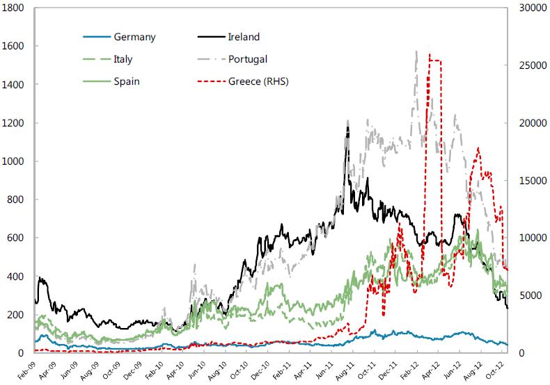
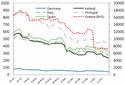
A. Data Description Table 1 reports stylized facts about the first two moments of the financial variables used in this study, while Figure 1 shows the raw series. The data frequency is daily and comprises the period from February 2, 2009 to April 9, 2010 initially, and extended first to July 18, 2012 and then to October 17, 2012. These periods capture the height of the buildup of the sovereign risk stage of the financial crisis that began in 2007 (IMF 2009, 2013).
After having validated kurtosis and the inexistence of unit roots for SCDS in first differences (with the marginal exception of the TED spread), we proceed to examine Granger-causality tests for the all the variables. The causality tests among financial variables are reported in Table 2 for the full sample.
B. Causality Tests The Granger-causality tests suggest that the global variables, TED spread and VIX, directly affect the German SCDS. Table 2 indicates that the statistical causality runs from TED, VIX, and all the other countries' SCDS spreads to the German SCDS. This conclusion seems intuitively plausible as German banks have invested or lent significant amounts to the other European countries. Global market indicators (such the VIX or the TED) would be expected to exert an overall influence on the German financial markets, and then be affected again through a second round by the financial turmoil coming from these countries. Based on the Granger causality analysis, and also because of earlier empirical studies discussed in the previous section, we proceed to model the German SCDS, using the TED, VIX and also the fiscally vulnerable countries' SCDS as exogenous explanatory variables. The various alternative models are discussed in the following sections.
Table 1. Stylized Facts for Sovereign Credit Default Swap, TED and VIX
(April 2009-July 2012)
Statistics Germany Portugal Ireland Italy Greece Spain TED Spread VIX Index Level Mean 54.8 519.2 437.3 245.2 3792.8 263.2 34.4 23.9 Standard Dev. 25.3 402.0 236.7 153.2 5786.3 149.4 21.4 7.9 Median 45.9 444.3 440.2 182.7 895.0 242.1 28.0 21.7 Min 19.0 44.5 114.7 56.6 100.3 54.8 10.6 13.5 Max 121.5 1581.7 1195.6 594.7 25960.8 642.4 112.9 52.7 5% Percentile 22.0 54.9 138.8 72.0 123.2 68.6 14.9 15.5 95% Percentile 102.2 1170.8 794.6 525.6 16141.0 541.0 95.7 41.2 Skewness 0.63 0.45 0.22 0.70 2.06 0.43 1.90 1.22 P-Value Skewness 0.0000 0.0000 0.0081 0.0000 0.0000 0.0000 0.0000 0.0000 Kurtosis-3 -0.77 -1.19 -1.14 -0.94 3.96 -0.78 3.49 0.99 P-Value Kurtosis 0.0000 0.0000 0.0000 0.0000 0.0000 0.0000 0.0000 0.0000 Autocorr 1 0.995 0.998 0.997 0.997 0.992 0.996 0.994 0.966 Autocorr 2 0.988 0.994 0.992 0.992 0.985 0.990 0.988 0.942 Autocorr 3 0.981 0.991 0.987 0.987 0.976 0.985 0.981 0.917 Partial AC 1 0.995 0.998 0.997 0.997 0.992 0.996 0.994 0.966 Partial AC 2 -0.201 -0.193 -0.218 -0.203 -0.004 -0.187 0.029 0.124 Partial AC 3 -0.013 0.032 0.003 0.085 -0.086 0.072 -0.042 -0.002 ARCH Test (T*R2) 920.91 933.71 921.87 927.64 921.68 938.80 955.11 800.36 P-Value 0.0000 0.0000 0.0000 0.0000 0.0000 0.0000 0.0000 0.0000 Unit Root (ADF) -2.06 -0.51 -0.40 -2.13 -3.46 -2.68 -3.83 -3.33 P-Value 0.5647 0.9828 0.9873 0.5297 0.0445 0.2455 0.0152 0.0623 First Difference
Mean 0.0 0.7 0.3 0.4 16.9 0.5 -0.1 0.0 Standard Dev. 2.9 27.5 20.0 14.7 759.1 15.1 1.3 1.9 Median 0.0 0.2 0.0 0.1 0.9 0.2 0.0 -0.1 Min -32.5 -184.0 -157.6 -72.5 -16477.5 -79.3 -9.0 -12.9 Max 33.3 383.8 315.2 236.8 9389.7 252.4 13.0 16.0 5% Percentile -3.8 -33.3 -23.6 -17.9 -344.8 -20.0 -1.9 -2.6 95% Percentile 4.0 35.7 25.5 20.5 395.9 20.4 1.8 2.9 Skewness 0.06 2.56 3.62 4.37 -8.24 4.56 0.54 0.96 P-Value Skewness 0.4611 0.0000 0.0000 0.0000 0.0000 0.0000 0.0000 0.0000 Kurtosis-3 37.19 45.61 70.29 72.47 259.12 81.71 15.07 12.34 P-Value Kurtosis 0.0000 0.0000 0.0000 0.0000 0.0000 0.0000 0.0000 0.0000 Autocorr 1 0.205 0.244 0.266 0.209 0.000 0.207 0.134 -0.145 Autocorr 2 0.057 0.006 0.053 -0.053 0.086 -0.056 0.053 0.005 Autocorr 3 -0.122 -0.090 -0.049 -0.140 0.030 -0.161 0.049 -0.167 Partial AC 1 0.205 0.244 0.266 0.209 0.000 0.207 0.134 -0.145 Partial AC 2 0.016 -0.057 -0.019 -0.101 0.086 -0.104 0.036 -0.017 Partial AC 3 -0.143 -0.082 -0.062 -0.113 0.030 -0.134 0.038 -0.173 ARCH Test (T*R2) 139.21 87.17 130.08 107.77 0.13 102.29 64.45 157.23 P-Value 0.0000 0.0000 0.0000 0.0000 0.9926 0.0000 0.0000 0.0000 Unit Root (ADF) -12.68 -10.31 -11.82 -19.80 -20.11 -18.51 -5.12 -7.99 P-Value 0.0000 0.0000 0.0000 0.0000 0.0000 0.0000 0.0001 0.0000 ADF: Augmented Dickey-Fuller test (automatic lags based on AIC); ARCH tests with 6 lags; P-Values for Skewness and Kurtosis from Normal distribution.
Table 2. Causality Tests for Sovereign Credit Default Swap, TED Spread, and VIX
(April 2009-July 2012)
Null Hypothesis F-Statistic Prob. Level
GREECE does not Granger Cause GERMANY 0.8500 0.5804 GERMANY does not Granger Cause GREECE 3.2792 0.0003 IRELAND does not Granger Cause GERMANY 2.6690 0.0032 GERMANY does not Granger Cause IRELAND 3.3526 0.0003 ITALY does not Granger Cause GERMANY 1.4028 0.1738 GERMANY does not Granger Cause ITALY 3.0625 0.0008 PORTUGAL does not Granger Cause GERMANY 2.6593 0.0033 GERMANY does not Granger Cause PORTUGAL 2.0616 0.0250 SPAIN does not Granger Cause GERMANY 1.5154 0.1286 GERMANY does not Granger Cause SPAIN 2.2414 0.0139 ITALY does not Granger Cause GREECE 2.8930 0.0014 GREECE does not Granger Cause ITALY 0.4469 0.9232 SPAIN does not Granger Cause GREECE 2.1279 0.0202 GREECE does not Granger Cause SPAIN 0.7053 0.7201 SPAIN does not Granger Cause ITALY 2.3037 0.0113 ITALY does not Granger Cause SPAIN 2.1390 0.0195 TED does not Granger Cause GERMANY 0.6917 0.7329 GERMANY does not Granger Cause TED 1.8407 0.0500 VTX does not Granger Cause GERMANY 1.7944 0.0575 GERMANY does not Granger Cause VTX 2.8989 0.0014 First Difference
DGRE does not Granger Cause DGER 0.9687 0.4691 DGER does not Granger Cause DGRE 2.1786 0.0171 DIRE does not Granger Cause DGER 1.6804 0.0807 DGER does not Granger Cause DIRE 2.7868 0.0021 DTT does not Granger Cause DGER 1.3916 0.1789 DGER does not Granger Cause DIT 3.6852 0.0001 DPOR does not Granger Cause DGER 1.5649 0.1121 DGER does not Granger Cause DPOR 2.4691 0.0064 DSP does not Granger Cause DGER 2.1531 0.0186 DGER does not Granger Cause DSP 2.6186 0.0038 DTT does not Granger Cause DGRE 1.7021 0.0757 DGRE does not Granger Cause DIT 0.6959 0.7289 DSP does not Granger Cause DGRE 1.3524 0.1978 DGRE does not Granger Cause DSP 1.2330 02653 DSP does not Granger Cause DIT 2.7683 0.0023 DTT does not Granger Cause DSP 2.3036 0.0113 DIED does not Granger Cause DGER 0.4643 0.9132 DGER does not Granger Cause DTED 1.1684 0.3084 DVTX does not Granger Cause DGER 1.7305 0.0696 DGER does not Granger Cause DVTX 2.8590 0.0016 Granger Causality Test with 10 lags Source: Authors' estimates.
Figure 1. Sovereign Credit Default Swaps, TED Spread, and VIX Index
(2009-2012)
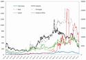
Click to enlarge
Note: The TED spread is in basis points, as are the CDS spreads. The VIX is an index.
III. Competing Empirical Models In this section, we estimate two classes of volatility models. First, several deterministic volatility specifications are estimated based on Bollerslev (1986) and Bollerslev (2008). A more complex stochastic volatility model is then estimated which is able to outperform previous deterministic models. The models are estimated using daily data in first differences, in order to account for stationarity in the data.
A. Deterministic Volatility Models This section presents some benchmark structures of deterministic volatility models widely used in financial empirical analysis. |14| Here, we first consider different symmetric GARCH models as benchmarks to examine the probability of sovereign default captured by SCDS. This is examined using a measure of risk based on the first difference of SCDS, or the logarithm of the square of the first difference of SCDS.
It is well documented that financial data exhibit heteroskedasticity (Engle, 2001) and instability (Galeano and Tsay, 2010). Most volatility models focus on financial variables (such as stock returns, interest rates, exchange rates, or commodity prices), while relatively few study macroeconomic variables (unemployment, inflation or growth).
The standard approach is as follows. The GARCH(1,1) specification (which is usually the benchmark in any deterministic volatility estimation) is represented by:
σt2 = ω + ρσ2t-1 + ϑε2t-1 (1)
where ρ, ϑ are the GARCH and ARCH coefficients, respectively. The usual non-negativity and additivity restrictions apply: ω > 0, ρ + ϑ < 1. Volatility is assumed to be determined in period t by two predetermined variables: a stochastic shock and the previous level of volatility which shows a certain degree ρ of persistence.
Given that most financial data exhibit a high level of kurtosis, we also consider the use of T-student distributions in our estimations. In this case the number of parameters includes also the degrees of freedom of the density function.
The results for selected representations are reported in Table 3, under the columns labeled I to IV. The results and analysis are discussed in Section IV below.
B. Stochastic Volatility Model The general structure of the basic stochastic model is represented by two blocks of equations which establish the state space system: the measurement equation (2), and the state equation (3).
yt = HBt + Axt + εty (2)
Bt= Γ0 + Γ1Bt-1 + εt (3)
Equation (2) represents the dynamics of the measurement variables defined by yt = ΔCDSt = CDSt - CDSt-1 (in our model, this represents the change in SCDS measured in basis points), which is explained by a vector of observed exogenous variables xt, a vector of unobserved state variables Bt, and an iid error term εty---iid---> N (0, Θ). For any measured variable the variance-covariance matrix is defined by Θ = σ2y < ∞, and it is estimated along with the other parameters. The estimations are performed using standard quasi-maximum likelihood (QML) procedures. |15|
The dynamics of the state variables are represented by the state equation (3). The error term in the state equation is assumed to be uncorrelated with the error term of the measurement equation, and in general is represented by a distribution centered on zero, normally distributed, and with a diagonal positive definite variance-covariance matrix Q.
εt---iid---> N (0, Q) (4)
The QML estimation is applied to the state space representation (2)-(4) using a Kalman filter approach. This is a recursive procedure based on two stages: prediction and correction. For prediction we use some prior information on estimates and variance-covariance matrices, while for the correction we use the posteriors on the estimates and the variance-covariance matrix. The Kalman factor makes use of prior information to generate the posteriors, and this learning procedure is iteratively repeated until all the sample data is analyzed. During the iteration process, optimization is performed to find the unknown parameters.
In our model, the State Space structure of the system can be represented by one measurement equation that links the current values of SCDS changes {yt} with two state variables labeled
as systemic risk and the idiosyncratic risk. In particular, the correlation of German SCDS with the SCDS for the fiscally vulnerable countries, which have recently exhibited higher sovereign risk, the TED spread and the VIX are used to account for global market conditions which proxy for systemic risk.
The stochastic nature of the volatility cannot be evaluated using deterministic approaches, such as GARCH models, including its variants (TGARCH, EGARCH, IGARCH, etc.). Starting from the stochastic volatility model presented in Shephard (1996), we expand the structure to include xt which constitutes the SCDS for the fiscally vulnerable countries, the TED spread, and the VIX index, as control variables for global market conditions (see, for example, Gonzalez-Hermosillo and Hesse, 2011).
Hence, the model is based on the following equations:
yt = γ J
∏
j-1xβjjt σt εt (5) ln σ2t = ω + ρ ln σ2t-1 + ηt (6)
εt ---iid---> N(0,1)
ηt ---iid---> N(0,σ2η)
From the non linear equation (5), we have the following measurement equation with the conventional linear representation:
y2t = γ2 J
∏
j=1x2βjjt σ2t ε2t (7) where j=1,...,7 represents the SCDS for the fiscally vulnerable countries, as well as the TED spread and VIX index (all variables in first differences).
Taking logs we get the final log-linear measurement equation:
ln y2t = μ + J
∑
j-1βj ln x2jt + ln σ2t + ζt (8) where μ = ln γ2, and ζt = ln ε2t. In the QML procedure we use: ζt ---iid---> N (-1.2704, π2/2). |16|
The model represented by equations (6) and (8) has the following State Space representation (using the (2)-(3) structure):
H = [1]
Bt =[ln σ2t]
A = [μ β1 β2 β3 β4 β5 β6 β7]
Θ = π2/2
Γ0 = [ω]; Γ1 = [ρ]
Variables y and x in our system are logs of squared first difference of German SCDS, other countries' SCDS, the TED spread and the VIX index, respectively, so they are measured in squared basis points. The residuals, as usual, follow Gaussian processes.
Finally, the variance-covariance matrix of the independent residual of the transition system is
as follows:
Q = [ρ2η] (10)
To conclude, an orthogonality condition between shocks is imposed:
Cov[ζt,ηt�s] = 0, ∀t, s (11)
In summary, the unknown parameters to estimate are {μ, β1, β2, β3, β4, β5, β6, β7, ω, ρ, σ2η}.
C. Stochastic Volatility Analysis As discussed, our analysis started with the traditional approach to analyze volatility estimating GARCH deterministic volatility models. Estimations are reported in Table 3.
To facilitate the analysis and discussion, we reproduce again equations (6) and (8):
ln σ2t = ω + ρ ln σ2t-1 + ηt (6)
ln y2t = μ +
J
∑
j=1βj ln x2jt + ln σ2t + ζt (8) IV. Model Results From Table 3, it is clear that the overall performance of the GARCH models is limited. In particular, the dynamics of deterministic volatility GARCH models show a strong sensitivity to the variance to the shocks, with unusual jumps not observed in the German SCDS spreads. Model I is the standard GARCH (1, 0), and model II includes the VIX and TED variables in the mean equation. Models III and IV are comparable to I and II respectively but now the implicit distribution for the likelihood is a T-Student and not a Normal Gaussian as in the first two models. Finally, model V represent the stochastic volatility structure with all the variables included. |17| Based on likelihood ratio tests (last segment in Table 3), this type of behavior is not supported by the data, which strongly supports the view concluding that stochastic volatility models outperform the traditional GARCH deterministic volatility models.
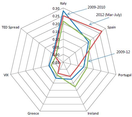
The significance of Italy and Spain's SCDS in determining Germany's SCDS is evident from the results (for example, Figure 2 shows the coefficients of the fiscally vulnerable countries which are very similar across alternative deterministic models). |18| This is also true for the stochastic volatility structure. All models have the same dependent variable so the log likelihoods are comparable. It is interesting to notice that for the measurement equations (first part of Table 3 the coefficients are quite similar: coefficients for Italy approximately 0.31 while for Spain around 0.15.
The Ireland and Portugal GARCH's coefficients are not significant, but once we introduce the T-Student distribution as a likelihood function, both parameters are significant at 10 percent. However, in the stochastic volatility model these coefficients are again not significant. In summary, some evidence of contagion from Portugal and Ireland to Germany exists but it is only marginal and not consistent across model specifications.
Another interesting result is that Greece is not significant in all the models, but Italy and Spain are consistently significant. The results suggest that the recent developments in Greece that led to the EC/ECB/IMF financial rescue of that country did not affect significantly the risk of Germany, at least not directly. |19| The parameter for Greece is slightly unstable, but always with the same sign, ranging from 0.0187 to 0.0631. Notably, this is different in the case of Italy and Spain as they appear to have a robust impact on Germany. The coefficients associated with Italy and Spain across all models are statistically significant. In the case of Italy, the estimated coefficients range from 0.28 (model V) to 0.32 (model I) and are significant at the 1 percent of significance level. For Spain, the coefficients are around 0.15-- 0.16 with a 5 percent of significance level in most of the estimated models. In terms of contagion from other sovereign European countries, these results suggest that for Germany the most important factors arise from Italy and Spain, and not from Greece, Ireland, or Portugal. |20| One possible explanation is that the problems in Greece were originally seen as stand-alone, though the generalized increase in the SCDS for other European countries is not supportive of this view. The other possibility is that Greece was seen as a country too small to affect Germany's risk. In contrast, Italy and Spain could potentially destabilize Germany, being much larger economies, even though their likelihood of running into financial difficulties was perceived by the market as comparatively small based on their SCDS.
The proxies for global non-Europe financial market conditions (VIX and TED) were not statistically significant across alternative model specifications. Even when the coefficients are stable ranging from 0.04 to 0.07 for the VIX and 0.03 to 0.04 for the TED spread, all results show a p-value of over 25 percent. The inclusion of these variables was rejected using a Likelihood Ratio (LR) test reported at the end of Table 3. |21| Comparing models I vs. II (which include VIX and TED) the LR test was 2.29 with a p-value of 13 percent not rejecting the null hypothesis that the joint coefficients are zero. This analysis was done also for the T-Student distribution comparing models III vs. IV (which includes VIX and TED). In this case the LR test was even lower reaching 1.68 with a p-value of 20 percent not rejecting the null hypothesis that the joint coefficients are zero. For the stochastic volatility (model V) the p-value of the VIX is 38 percent while for the TED spread the p-value was 40 percent, hence in both cases we do not reject the null hypothesis that each coefficient is zero.
Analyzing the volatility equation (6) for the deterministic models I-IV, the autocorrelation coefficient p is estimated robustly at 0.98--0.99 with very low standard deviations and with low P-values (0.0000), rejecting the null hypothesis that those parameters are zero. The stochastic volatility models V-VII have statistically significant estimated standard deviation coefficients. Its estimated value is in the range of about 0.67--1.61 with a p-value of 0.46 percent or 0 percent (below 1 percent) which supports strongly the hypothesis of a stochastic volatility structure. This is confirmed by a LR test between our benchmark deterministic model II and the stochastic volatility model V, reporting a chi-square test of 7.19 with a p-value of 0.73 percent, below the 1 percent threshold (see last segment of Table 3).
Table 3. Estimation Results for the German Sovereign Credit Default Swap Spreads: Volatility Models
Parameters I II III IV V1/ VI1/ VII1/ Y -1.8781 -1.7619 -1.6444 -1.5614 2.5951 -1.1797 -1.1833 Std. Error 0.1921 0.2160 0.1520 0.1610 1.8610 0.2042 0.2100 Test -9.7789 -8.1583 -10.8204 -9.7011 1.3944 -5.7772 -5.6335 P-Value 0.0000 0.0000 0.0000 0.0000 0.1665 0.0000 0.0000 Portugal 0.0886 0.0914 0.0882 0.0930 0.0849 0.1066 0.1067 Std. Error 0.0638 0.0635 0.0462 0.0465 0.0670 0.0382 0.0385 Test 1.3876 1.4390 1.9064 2.0019 1.2685 2.7906 2.7693 P-Value 0.1685 0.1535 0.0597 0.0482 0.2078 0.0064 0.0068 Ireland 0.0936 0.0905 0.0754 0.0757 0.0717 0.1261 0.1261 Std. Error 0.0636 0.0631 0.0403 0.0403 0.0480 0.0400 0.0412 Test 1.4716 1.4348 1.8697 1.8765 1.4945 3.1525 3.0632 P-Value 0.1445 0.1547 0.0646 0.0637 0.1384 0.0022 0.0029 Italy 0.3195 0.3158 0.3003 0.2939 0.2810 0.2143 0.2142 Std. Error 0.0821 0.0820 0.0519 0.0519 0.0710 0.0499 0.0500 Test 3.8908 3.8494 5.7890 5.6661 3.9552 4.2946 4.2869 P-Value 0.0002 0.0002 0.0000 0.0000 0.0001 0.0000 0.0000 Greece 0.0187 0.0198 0.0438 0.0469 0.0631 0.0405 0.0405 Std. Error 0.0645 0.0644 0.0463 0.0462 0.0597 0.0208 0.0212 Test 0.2896 0.3078 0.9461 1.0153 1.0573 1.9471 1.9138 P-Value 0.7727 0.7589 0.3465 0.3126 0.2931 0.0545 0.0587 Spain 0.1585 0.1520 0.1524 0.1534 0.1592 0.1732 0.1732 Std. Error 0.0774 0.0778 0.0548 0.0547 0.0715 0.0460 0.0467 Test 2.0475 1.9540 2.7813 2.8041 2.2258 3.7652 3.7061 P-Value 0.0434 0.0537 0.0065 0.0061 0.0284 0.0003 0.0004 VIX 0.0714 0.0474 0.0429 0.0301 0.0301 Std. Error 0.0655 0.0419 0.0488 0.0271 0.0336 Test 1.0903 1.1306 0.8794 1.1107 0.8984 P-Value 0.2784 0.2611 0.3814 0.2695 0.3713 TED Spread 0.0350 0.0255 0.0367 0.0111 0.0111 Std. Error 0.0464 0.0546 0.0438 0.0173 0.0258 Test 0.7542 0.4674 0.8386 0.6416 0.4313 P-Value 0.4526 0.6413 0.4038 0.5227 0.6672 Volatility
Unconditional Volatility2/ 2.1700 2.1569 1.9351 1.9607 1.6090 3.2290 3.2308 ω 0.0648 0.0592 0.0277 0.0266 -0.8158 -0.0060 -0.0044 Std. Error 0.1466 0.1505 0.0623 0.0744 0.7771 0.0164 0.0300 Test 0.4422 0.3934 0.4451 0.3570 -1.0499 -0.3659 -0.1471 P-Value 0.6594 0.6949 0.6573 0.7219 0.2965 0.7153 0.8834 ρ 0.9862 0.9873 0.9926 0.9931 0.7380 0.5552 0.5552 Std. Error 0.0250 0.0262 0.0121 0.0146 0.1391 0.0640 0.0640 Test 39.424 37.701 82.250 68.001 5.3071 8.6750 8.6704 P-Value 0.0000 0.0000 0.0000 0.0000 0.0000 0.0000 0.0000 σ_η 0.6704 1.6091 1.6091 Std. Error 0.2308 0.1284 0.1284 Test 2.9052 12.5319 12.5310 P-Value 0.0046 0.0000 0.0000 DoF T-Distr. 5.2252 5.2919 Std. Error 1.2640 1.2742 Test 4.1337 4.1530 P-Value 0.0001 0.0001 Systemic Risk3/ 22.5% 23.0% 21.4% 22.9% 23.9% 22.3% 22.3% Idiosyncratic Risk 77.5% 77.0% 78.6% 77.1% 76.1% 77.7% 77.7% Log-Likelihood4/ -708.83 -707.69 -689.42 -688.58 -704.09 -2224.24 -2224.24 Test LR Test 2.2900 1.6782 7.1895 P-Value 0.1302 0.1952 0.0073 Testing Models I - II III - IV II - V 1/In all models sample starts at 2009. Model V sample ends 2010; Model VI sample ends July 2012; Model VII data ends in Oct 2012.
2/The unconditional volatility for the SV model is the sum of the stochastic volatility and the deterministic variance.
3/Correlation between the model and the observed data.
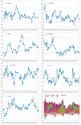
4/In Model VII the Log-likelihood statistic was computed using 2012 (May-July) data.Figure 2. Determinants of German Sovereign Credit Default Swap Volatility:
Stochastic Volatility Model
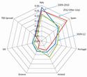
Click to enlarge
Source: Estimates from volatility regressions (Table 3).
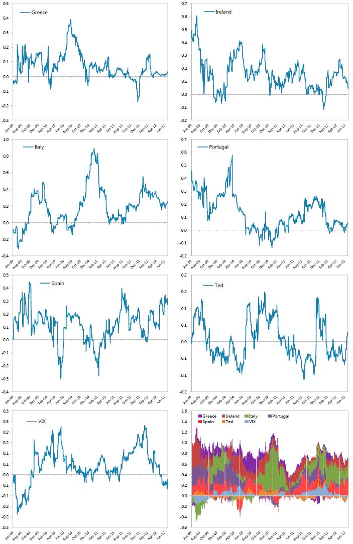
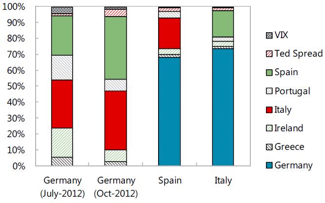
A. Stability Analysis To test for stability and the relative determinants of the SCDS volatilities, we estimate the coefficients of the model using a rolling window sample (size of 100 days) starting from February 2009 (Figure 4). The importance of Italy and Spain was also revealed using this methodology. As shown in Figure 2, Spain has been increasing its relevance lately in explaining the Germany's SCDS dynamics. However, Italy's influence is still very high.
In sum, a remarkable finding of this paper is the persistent and almost permanent effect that extreme bad news have on the stochastic volatility and, consequently, on the change in SCDS spreads. For Germany, changes in the credit ratings of Greek sovereign debt, including news announced in the first quarter 2010 related to Greece's bailout package, had no statistical effect on the country's SCDS. It is also interesting to note that the global non-European measures used as proxies for global market conditions (VIX and TED spreads) were not statistically significant in explaining Germany's SCDS dynamics (see Figure 2). Indeed, the results suggest that Germany's SCDS fluctuations are determined not only from idiosyncratic risk and its own macroeconomic and financial characteristics, but also by market developments in some of the bigger economies in Europe such as Italy and Spain. These dynamics are also sustained based on the stability analysis done with rolling windows of daily data (see Figure 4). Trends for Greece and Ireland are showing the relatively low importance of these two countries in explaining Germany's SCDS fluctuations, while Italy and Spain explain most of the dynamics, especially during the last segment of the sample as shown in the bottom right panel of Figure 4.
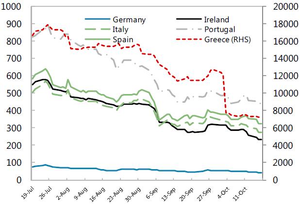
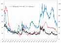
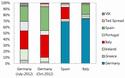
B. Extending the Model Through October 2012 and Explaining Spanish and Italian Sovereign Credit Default Swap In this section we extend the model to include the analysis of two other countries in the European region as independent variables: Italy and Spain. Using data through October 2012, we proceed to estimate the stochastic volatility model for Germany using the same structure and systemic variables discussed above, and we estimate the same volatility structure for Spain and Italy. The more recent developments in international financial markets show a generalized decline in the SCDS (especially for Greece after it defaulted on its sovereign debt).
Figure 3. Sovereign Credit Default Swaps
July-October 2012
Click to enlarge
The update of the model with data extending from July 2012 to October 2012 reinforces the conclusion that Italy and Spain are the only countries that help explain Germany's SCDS volatility, while Greece, Ireland, and Portugal remain relatively unimportant. As before (see Table 3), systematic risk accounts only 22 percent of the German SCDS volatility with the remaining volatility explained by idiosyncratic characteristics.
We also extend the analysis done for Germany for Italy and Spain. Not surprisingly, Germany plays a central role in explaining volatility in those fiscally vulnerable countries SCDS (Figure 4). For Spain, almost � of its volatility is explained by Germany's SCDS, while the remaining systematic risk comes from spillovers from the Italian SCDS. Similarly, most of Italy's systematic risk is explained by Germany, but also Spain plays an important role. As in the case of Spain, VIX, TED and other countries spillovers do not help significantly explain systemic risks in Italy.
Figure 4. Volatility Decomposition Using Rolling Window Data
(2009-2012)
Click to enlarge
Figure 5. Volatility Decomposition: Germany, Italy, and Spain
Click to enlarge
V. Conclusion The financial crisis has had an impact on the entire world, particularly as a result of spillovers and contagion. In an attempt to discern how much of the pressure that seemed to spread around European markets was either systematic or idiosyncratic, this paper focuses on these two factors for the case of Germany as the largest European economy. The analysis is based on SCDS spreads as a measure of the probability of sovereign distress. By modeling the dynamics of SCDS markets with stochastic volatility models we are able to determine the relative magnitudes of two types of risks: systematic and idiosyncratic.
Using SCDS spreads for Greece, Ireland, Italy, Portugal and Spain, and TED spreads and the VIX index as proxies for different aspects of global market conditions, we are able to assess the dynamics of the German SCDS market. For Germany, the results suggest that global non-European risk factors are statistically insignificant with no obvious contribution from the TED spread or the VIX index. Remarkably, Germany's SCDS dynamics appear to be driven not only by idiosyncratic risk and its own macroeconomic and financial conditions, but also by market developments in Italy and Spain. These countries are some of the largest countries in Europe within our data sample which may explain their pivotal role in determining Germany's SCDS spreads and, likely, the stability of the entire euro area.
Additionally, it is shown how stochastic volatility is significant in determining the dynamics of SCDS markets. Instead of assuming a finite number of volatility states (for example, in traditional regime-switching models), our stochastic volatility approach is more flexible as discrete jumps in volatility are replaced by smooth pass-through to SCDS spreads. The estimation reveals that the data generating process for stochastic volatility for the SCDS sample considered is highly persistent.
In summary, in our most general specification we observe that, for the case of Germany, most of the total measured volatility comes from idiosyncratic risks. The second source of volatility originates from European market conditions, coming mainly from Italy and Spain. Remarkably, macroeconomic or financial disturbances from other countries such as Ireland, Portugal or even Greece were not significant in explaining Germany's SCDS volatility. When we extend the results to explain the SCDS for Spain and Italy, we find that Germany's SCDS are very important in explaining their respective volatility, which is not surprising given the predominant role of Germany as the core country in Europe and the fact that this country is considered the risk-free benchmark for sovereign markets in Europe. Interestingly, these countries are also not significantly affected by Greece or any of the global market factors selected such as the TED spread or the VIX (similar to the results for Germany's SCDS). However, both Italy and Spain show significant co-dependence in explaining each other's SCDS volatility.
Finally, as a future extension of this paper, this methodology can be useful in other applications to support macroprudential policies. For example, it could be applied to produce an early warning indicator of financial stress, as volatility can be decomposed between solvency and liquidity factors.
[Source: By Brenda González-Hermosillo and Christian Johnson, International Monetary Fund, Monetary and Capital Markets Department, Apr14]
Arezki, Rabah, Bertrand Candelon, and Amadou N. R. Sy, 2011, "Sovereign Rating News and Financial Markets Spillovers: Evidence from the European Debt Crisis," IMF Working Paper No. 11/68 (Washington: International Monetary Fund). Beirne, J. and M. Fratzcher, 2012, "The Pricing of Sovereign Risk and Contagion during the European Sovereign Debt Crisis," European Central Bank. Berndt, A., and I. Obreja, 2010, "Decomposing European CDS Returns." Review of Finance, Vol. 14, pp.189-233. Blanco, R., S. Brennan, and I. Marsh, 2005. "An Empirical Analysis of the Dynamic Relation between Investment-Grade Bonds and Credit Default Swaps." The Journal of Finance, Vol. LX, No. 5, pp. 2255-81. Bollerslev, T., 1986, "Generalized Autoregressive Conditional Heteroskedasticity," Journal of Econometrics, Vol. 31, 307-27. ______, 2008, "Glossary to ARCH (GARCH)," CREATES Research Paper, pp. 2008-49, School of Economics and Management, University of Aarhus, Denmark. Caceres, C., V. Guzzo, and M. Segoviano, 2010, "Sovereign Spreads: Global Risk Aversion, Contagion or Fundamentals?" IMF Working Paper No. 10/120 (Washington: International Monetary Fund). Carr, P., and L. Wu, 2009, "Stock Options and Credit Default Swaps: A Joint Framework for Valuation and Estimation," Journal of Financial Econometrics, Vol. 8(1), pp. 1-41. Collin-Dufresne, P., R. Goldstein, and J. Martin, 2001, "The Determinants of Credit Spread Changes." The Journal of Finance, LVI(6), pp. 2177-207. Di Cesare, Antonio, Giuseppe Grande, Michele Manna and Marco Taboga, 2012, "Recent Estimates of Sovereign Risk Premia for Euro-area Countries," Questioni di Economia e Finanza, Banca D'Italia Eurosisema, September, Number 128. Dornbush, R., Y.C. Park, and S. Claessens, 2000, "Contagion: Understanding How It Spreads," The World Bank Research Observer, 15(2), pp. 177-97. Dungey, Mardi, Renee Fry, Brenda Gonzalez-Hermosillo, and Vance Martin, Transmission of Financial Crises and Contagion: A Latent Factor Approach, 2011, Oxford University Press publishers, U.K. ______, 2005, "Empirical Modeling of Contagion: A Review of Methodologies," Quantitative Finance, Vol. 5, No. 1, February. Engle, R., 2001. "GARCH 101: The Use of ARCH/GARCH Models in Applied Econometrics." Journal of Economic Perspectives, Vol. 15(4), pp. 157-68. Espinoza, R., and M. Segoviano, 2011, "Probabilities of Default and the Market Price of Risk in a Distressed Economy," IMF Working Paper No. 11/75 (Washington: International Monetary Fund). Favero, C.A., 2013, "Modelling and Forecasting Government Bond Spreads in the Euro Area: a GVAR Model," memo, February. Forbes, K., 2012, "The 'Big C': Identifying Contagion," NBER Working Paper No. 18465, (Cambridge, Massachusetts: National Bureau of Economic Research). Forbes, K., and Rigobon, R., 2002, "No Contagion, Only Interdependence: Measuring Stock Market Co-movements," Journal of Finance, Vol. 57(5), pp. 2223-61. Galeano, P., and R. Tsay, 2010, "Shifts in Individual Parameters of a GARCH Model," Journal of Financial Econometrics, Vol. 8(1), pp. 122-53. González-Hermosillo, B., and H. Hesse, 2011, "Global Market Conditions and Systemic Risk," Journal of Emerging Market Finance, Vol. 10, Number 2, August. Harvey, A. C., E. Ruiz, and N. Shephard, 1994, "Multivariate Stochastic Variance Models," Review of Economic Studies, Vol. 61, pp. 247-64. International Monetary Fund (IMF), 2009, "Detecting Systemic Risk," In Global Financial Stability Report, Chapter 3 (Washington, April). _____, 2013, Global Financial Stability Report, Chapter 2. (Washington, April). Johnson, C., 2011, "Determinants of Credit Default Swaps Using a Stochastic Volatility Model," Unpublished manuscript. Kim, M., B. Jang, and H. Lee, 2008, "A First-Passage-Time Model under regime-Switching Market Environment," Journal of Banking and Finance, Vol. 32, pp. 2617-27. Lekkos, I., 2007, "Modeling Multiple Term Structures of Defaultable Bonds with Common and Idiosyncratic State Variables," Journal of Empirical Finance, Vol. 14, pp. 783817. Longstaff, F., S. Mithal, and E. Neis, 2005, "Corporate Yield Spreads: Default Risk or Liquidity? New Evidence from the Credit Default Swap Market," The Journal of Finance, Vol. LX, No. 5, pp. 2213-53. Sgherri, S., and E. Zoli, 2009, "Euro Area Sovereign Risk During the Crisis," IMF Working Paper No. 09/222 (Washington: International Monetary Fund). Shephard, N., 1996, "Statistical Aspects of ARCH and Stochastic Volatility," In Time Series Models In Econometrics, Finance and Other Fields, eds. D.R. Cox, D. V. Hinkley, and O. Barndorff-Nielsen, London: Chapman & Hall. Yibin, B., H. Zhou, and H. Zhu, 2009, "Explaining Credit Default Swaps Spreads with the Equity Volatility Jump Risks of Individual Firms," The Review of Financial Studies, Vol. 22, No. 12, pp. 5100-31.
Notes:
1. The authors are grateful for useful discussions and comments received from participants at seminars organized at the Massachusetts Institute of Technology and at the IMF. Without any implication, we would also like to thank Antonio Bassanetti, Gaston Gelos, Laura Kodres, and Fernando Varela for useful comments. [Back]
2. The rationale for this policy is examined analytically in IMF (2013), where it is argued that the recent ban "appears to move in the wrong direction." [Back]
3. See, for example, Dungey, Fry, Gonzalez-Hermosillo, and Martin (2011), Dornbush, Park, and Claessens (2000); Forbes and Rigobon (2002); Sgherri and Zoli (2009); and Arezki, Candelon, and Sy (2011). [Back]
4. Various technical approaches are contrasted empirically in Dungey, Fry, Gonzalez-Hermosillo, and Martin (2011). They show that some of the most influential empirical techniques that have been used are either equivalent or a special case of a more general latent factor approach. A recent survey of contagion is provided in Forbes (2012). [Back]
5. See, for example, González-Hermosillo and Hesse (2011). [Back]
6. Based on Depository Trust and Clearing Corporation (DTCC) data; see IMF (2013). [Back]
7. Other related research examining sovereign risk premia in the euro area include Favero (2013) and Di Cesare and others (2012). [Back]
8. See, for example, Kim et al. (2008), and Dungey et al. (2005). [Back]
9. As determinants of changes in SCDS they include changes in interest rates (10-year bond yields), changes in slope of the yield curve (change in spreads on 10- and 2-year Treasury bonds), changes in equity prices (S&P 500 and Stoxx index), and changes in the implied equity volatility (near-the-money put options). [Back]
10. Using U.S. and U.K. corporate bond data, Lekkos (2007) estimates a reduced form of a dynamic factor model for the interest rate term structure of defaultable bonds which include common factor variables. Variables used to measure the credit cycles' indicators included: the slope of the term structure (10-year vs. 3-month U.S. Treasuries), the level of the term structure (changes in the 3-month U.S. Treasury bill rate), the spread between Libor and the U.S. Treasury bill (TED spread), interest rate swap spreads (3-, 7- and 10-year swaps), and equity returns (Financial Time Stock Exchange, FTSE-100 for the U.K. and S&P500 for the U.S.). [Back]
11. Using a regime-switching model, Gonzalez-Hermosillo and Hesse (2011) proxy global market conditions using three variables: VIX index, TED spreads and the Euro-Dollar Foreign Currency Swap. [Back]
12. Using a panel of corporate firms across January 2001 to December 2003, this paper explains the CDS premium using as explanatory variables the credit ratings, recovery rate used by CDS price providers, return on equity, firm leverage, dividend payout ratio and global market conditions such as S&P 500, VIX index, TED spread and the short interest rate. [Back]
13. Caceres et al. (2010) and Espinoza and Segoviano (2010) develop a methodology to strip out the price effect of risk aversion. Also, it is common practice to get the probabilities of default by dividing the level of the SCDS by its recovery rate. This methodology can be considered as an extension of this paper. [Back]
14. For a summary of volatility models see Bollerslev (2008). [Back]
15. The computer code was written in GAUSS using the Constrained Maximum Likelihood procedure (CML), and is available upon request. [Back]
16. See Harvey and others (1994). [Back]
17. GARCH (1,1) structures report in general similar results. [Back]
18. See estimates on Table 3. [Back]
19. As an extension, a multivariate stochastic volatility model could be considered to control for all kind of indirect effects. [Back]
20. Alternative specifications with lags of the exogenous variables as explanatory variables report similar results, not changing the conclusions. [Back]
21. Causality between VIX or TED and SCDS spreads is generally low so the insignificance of VIX and TED in the volatility equations is not result of hidden indirect causalities. [Back]
 | This document has been published on 13May14 by the Equipo Nizkor and Derechos Human Rights. In accordance with Title 17 U.S.C. Section 107, this material is distributed without profit to those who have expressed a prior interest in receiving the included information for research and educational purposes. |